Hi everyone
I wrote a simulation program to calculate the coincident time resolution of LYSO detector. There is one point source emitting 511 keV radiation isotropically and two LYSO detectors of size 2.7x2.7x18 mm. I defined a scorer as a cathode at the end of the scintillator and saved the global time when optical photons entered the scoring volume. I am attaching the code snippet below. I was expecting the FWHM of difference of time (photonTime-photonTime1) captured to be in range of 100s of picosecond but rather I was getting it to be around 4 ns, which is quite high. Am I doing it correctly or what is wrong here ? Kindly let me know.
if(stepstatus==fGeomBoundary){
		// check if the photon is absorbed in the sensitive volume
	if (currentPhysicalName == "Cathode"){

			if (particleName == "opticalphoton"){

			  photonTime = aStep -> GetPreStepPoint() -> GetGlobalTime();

		       	outFile.open("cathodelnew.data", std::ofstream::app);

 outFile  <<std::setprecision(15)<<photonTime/s << " "<<evt1<<std::endl;
 outFile.close();
		}
	}
	}

	if(stepstatus==fGeomBoundary){
	if (currentPhysicalName == "Cathode1"){

		if (particleName == "opticalphoton"){

			  photonTime1 = aStep -> GetPreStepPoint() -> GetGlobalTime();

			outFile.open("cathodel1new.data", std::ofstream::app);

 outFile <<std::setprecision(15)<<photonTime1/s << " "<<evt1<<std::endl;
 outFile.close();
		}
	}
}}
Scintillation photons are emitted after some time. What are your material parameters that specify this time?
Optical photons can bounce around forever. Maybe look at verbose tracking or visualization for some of your detected photons and try to understand the absolute times first, before the difference. (if you have, then let us know).
I am not sure about verbose tracking yet. But as shown in the code snippet, I find individual time and then subtract it. The individual time looks like this. Just including 10 values. The value after space is event number.
Oh I see this. But then, what should I put here on this property? This is the actual value of the decay constant of LYSO. If that’s the case then how I can get picosecond scale of resolution ?
Kindly help
I also request @John_McFee , @weller , @bmorgan, @mkelsey and other experts in the field to provide some insights if possible. I have been stuck on this for a while and unable to figure it out. Your help will be highly appreciated.
You are measuring the arrival time at the photocathode of the optical photons from scintillation. That is dictated by the scintillator decay constant and the optical geometry. So it its distribution should be roughly an expoential with a time constant similar to the decay constant. The “range of 100 ps” that you expect is for the FWHM from a timing coincidence experiment. Methods vary, but they all involve triggering very close to the beginning of a pulse or at a fixed fraction of the pulse height (e.g., search “constant fraction discriminator”). As such, the time distribution is much narrower than the decay time distribution. I suppose you could simulate that in Geant4, but off line analysis is likely easier.
Thank you so much for the reply.
I actually read it in an article about calculating the average time when the photons reach the scorer to calculate intrinsic time resolution.
"
To obtain the ITR of each configuration, we obtained the ATvalue, this value represents the average time at which the optical photons reach to the Scorer and it is obtained event byevent
I’ll have to read the paper in detail, but at first glance it seems to me that the method you describe will yield a time difference with uncertainty of the order of the decay time constant. The response from each detector is exponentially distributed (P=1/lambdaexp(-lambdat) where lambda = 1/35ns). The variance of the time of arrival of one detector is 1/lambda^2 and the variance of the time difference between the two detectors (assuming they are the same) is 2/lambda^2. So the standard deviation of the time difference between the two detectors should be ~1.4*36ns.
I understood your point. Thanks for the detailed description, How does people finding CTR perform the simulation, this is still a little unclear to me. But thank you for your response.
There is a digitization package in Geant4 (See Digitization in the Users Guides) which can be used to simulate some of the aspects of a signal processing chain (ADCs. TDCs, readouts, trigger logic, etc.), but I am not familiar with it. I’ll let the experts comment on it further. You can analyze the time response outside Geant4, which is generally my preference.
If you save the arrival time of optical photons that arrive at the PMT front face and their corresponding event number in a file you have exactly what a PMT photocathode would “see” event by event. One should be able to use fast prototyping software like Matlab or Octave to analyse that to simulate pretty much any signal processing technique ypu can think of (e.g., single photon detection, threshold detection, CFD, etc.). A number of those will have significantly better time resolution than one would get from the raw scintillation decay signal.
I am also working on the same idea as you are, simulating the time response of a scintillation detector, and would like to validate my results against published experimental data. In my simulation, I have defined the properties of the scintillating material, generated optical photons, and verified their production statistics. I have also implemented a photocathode to obtain the arrival-time distribution of these photons.
I understand that delays due to the material’s intrinsic properties—such as rise time, decay time, light yield, and photon transport—are already included in the scintillator model. However, I am unsure how to correctly handle the electronics response (e.g., photodetector timing characteristics, signal shaping, or electronic jitter) within the simulation to achieve realistic timing results.
Could anyone suggest methods or best practices for incorporating or validating the electronics component of the timing response when comparing simulation results with published data?
Geant4 handles the intrinsic physics of radiation and light transport. Generally the cleanest approach is to use the output of Geant4 as an input to another modelling/simulation code to handle the electronics since it will provide the “ground truth” arrival times. Timing thresholds tend to be best when set as close to the single photon detection limit as possible. Series and parallel electronic noise, crosstalk, dark counts, etc. act as sources of rising edge jitter.
You can find many papers attempting to model this response as “sipm waveform modelling” or “PMT waveform modelling” and specifically the single photon limit. GATE, a wrapper for Geant4, does this “under the hood” with its digitizer module. But again you will notice it just takes parameters for the noise sources. Detailed modelling would likely use PSpice or other circuit analysis software. Or you could just bootstrap it by building a single unit with smaller crystal and the devices you want to test and just measuring them. More costly, but less prone to bias.
Thanks for the reply. I understand a little from your answer that I should take the arrival time of photons at the photodetector and then take this information as input to model the electronics part using other models. But I am a bit confused. Like, for an event, I have the number of photons. For example, let’s consider 200 photons that enter the photodetector for a single event. All these photons have different arrival times, so for this event, for which photon do I have to store the time? And at what time should I store the information? That means when the photon is absorbed in the photodetector, or when it just hits the surface of the photodetector?
There are many ways to go about doing this. And it is usually an iterative process unless you are locked into a particular photosensor or readout electronics. As a starting point you could do the following:
Determine or estimate the noise floor of your readout circuit in terms of single photon amplitudes (almost all photosensors nowadays have single photon sensing), call it N.
In your geant simulation track the time when the optical photons are first generated or when they escape the surface with your photosensor. The second will be more accurate but require turning on and correctly setting up optical interfaces of your system.
Record only the first 1 - 2N photon timestamps, spaced as a tradeoff between the size of the output file versus usefulness. This could be done with a vector or array that you save in your end of event step. If N is 10, then 1-20. If N is 100, then maybe 1, 10, 20, …190, 200. Recording values below your noise/trigger floor will let you see what advantages you might gain from developing lower noise readout circuits (a non trivial task and cost increase). Generally speaking the “earlier” photon you are able to use the less overall jitter.
Use these events and the photon arrival times as input to a circuit model or simulation. This would not be in Geant4. In addition to modelling the electronic noise you can also model photosensor noise effects for higher accuracy including dark counts, afterpulsing, and crosstalk. For timing purposes, dark counts dominate while afterpulsing and crosstalk will dominate at higher event rates.
The idea is that you can create distributions of “arrival” times using which number of photons. You sample from these distributions to generate time stamps. At each point you can then place a single photon waveform and add them together (typically they have tails that sum together). Add random uncorrelated noise from the electronics and dark counts to the waveform and correlated noise if you want higher precision (afterpulsing, cross talk). Then feed those artificial waveforms back into your electronics or just set thresholds on the waveforms. What you should find is that the ideal trigger threshold will not be N but N + C where C is found as a tradeoff between lower jitter and baseline noise.
Hi, @jrellin@John_McFee
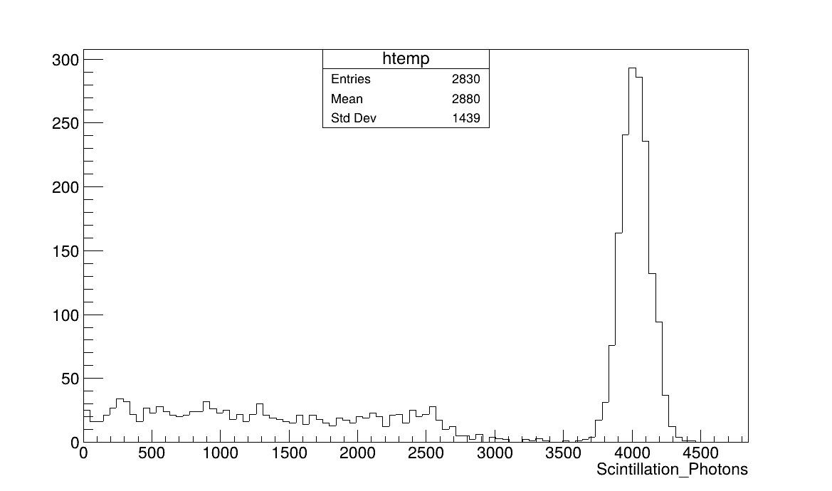
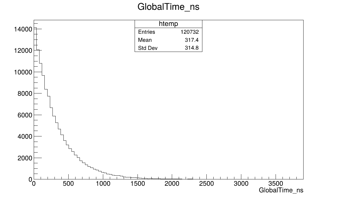
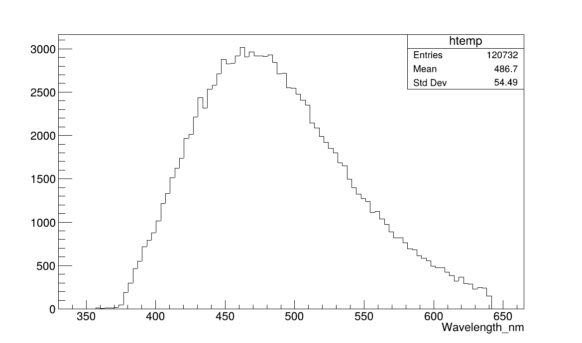
My goal is to build a simulation that gives me the detector time resolution. As in the lab, when we conduct an experiment, we use a time-correlated single-photon counting setup to determine the detector’s time resolution. Which is defined experimentally as follows: we have a source to irradiate a scintillator, which does the Compton and photoelectric effect and produces secondary electrons that further produce optical photons, and we place a photodetector to detect the optical photons and then amplify the signal and get the final waveform on the oscilloscope. A direct trigger is given to the oscilloscope from the same source that we use to irradiate the scintillator. We take the time difference between trigger arrival time and signal arrival time, which gives delta t, and then apply a Gaussian or convolution between Gaussian and exponential to find FWHM, which is the detector time resolution. In my simulation, I successfully defined the optical properties and produced optical photons. Figure 1 shows the production of scintillating photons as I am using a BGO scintillating crystal, and I verify this with the energy deposition distribution; the number of scintillating photons is correct. Now the problem is with designing and implementing the model for detector time resolution. For this purpose, I placed a SIPM on the opposite face of the scintillating crystal from the face where the source is placed and tracked the global time of optical photons that were absorbed inside the SIPM. I have attached the global time distribution of these optical photons that were absorbed into the SIPM. Now I am confused about how to verify whether this distribution is correct or not. For BGO, the decay time is 317 ns. One more thing that is confusing me: I run a simulation for 5000 events, out of which almost 2830 events produced optical photons, and out of these events, 2626 events have the photons that are absorbed into SIPM. Now my question is that when I have to take data for adding electronic noise from other software or models out of Geant4, what information should I have to use as input?
Figure 1. Scintillating Photons at the creation level
For modelling time resolution your time of arrival plot, assuming its all photons, is as far as Geant4 could take you and it looks, at first glance, as accurate or reasonable. For next steps, it depends on how details you want to be.
A simpler model would:
Model the Time of arrivals as delta pulses for the average number of photons per photopeak event
Sort the list, take the first, second, third, etc. times as the ideal trigger time and create distributions with ground truth resolution Tg
A more sophisticated model would then:
Model the waveforms for the single photons using models such as in Figure 5 here.
The inputs - quench resistance, microcell, etc. - are specific to your SIPM from the data sheet. Capacitance will add the more SIPMs are in parallel (degrading your time constants).
Add them together to generate noiseless waveforms to test your pickoff.
Another layer would be:
Add dark count events. These are indistinguishable from photon events. They are randomly distributed in time at a rate that is temperature and overbias dependent (from the data sheet).
Add after pulsing. This would be a probability that the Xth photon generates another photon at a later time T. This is ignorable if your event rate is not too high.
Cross talk. The data sheet will have internal crosstalk but the external crosstalk would require possible another simulation since its dependent on the crystal and wrapping above it.
The last step would be to add electronic noise to the waveforms. This will be driven by your readout circuit. This would either have to be done in a circuit simulator software or measured.