I am simulating the particle induced background of a X-ray telescope in space. I used GPS for the particle source and used Sensitive Detector to obtain background counts on the microcalorimeters. In particular, I used a biased sphere and a cosine law angular distribution. The macro file I used is
# Set the position of the source
/gps/pos/type Surface
/gps/pos/shape Sphere
/gps/pos/centre 2575.0 -5437.5 -25.0 mm
/gps/pos/radius 500 cm

/gps/hist/type biaspt # Account for the Earth occultation
/gps/hist/point 0. 1.
/gps/hist/point 0.6609 1.
/gps/hist/point 1. 0.

# Set the angular distribution of the source
/gps/ang/type cos
/gps/ang/mintheta 0 deg
/gps/ang/maxtheta 11.53 deg # sin 11.53 = 0.2
Then I did the normalization procedure in Section 3.2 of Fioretti et al. 2012 which normalizes the hit counts to background count rate. The procedure is
total_flux = integrate.quad(lambda x: PrimaryParticleFlux('proton',x / 1e3, phi=phi, thetaM=thetaM, h=h)*1e-4, energy_lower, energy_upper)[0] # in unit of counts cm^-2 s^-1 sr^-1
particle_rate = total_flux * 4 * np.pi**2 * (source_radius*np.sin(theta_max))**2 # in unit of counts s^-1
particle_rate = particle_rate / 2 * (1-np.cos(np.deg2rad(horizon_angle))) # correct for the Earth occultation
time = num_event / particle_rate # in unit of s
bkg_rate_integral = hits / time / effctive_area # in unit of counts s^-1 cm^-2
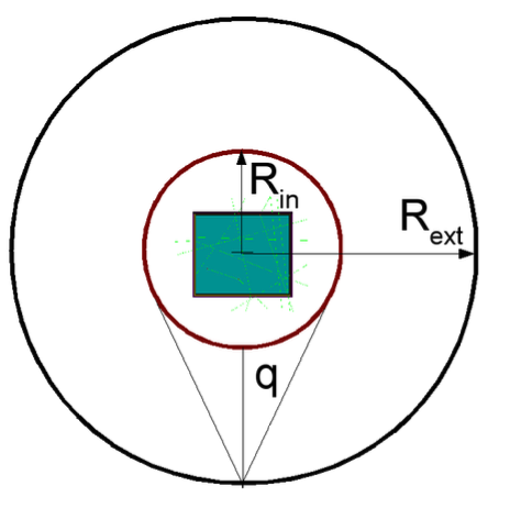
If I had it right, the background count rate should be uncorrelated with either the source sphere radius R_ext (i.e. source_radius) or the half cone angle q (i.e. theta_max). However, in my simulation, I found that the background count rate did change with the change of R_ext and q. Specifically, the background count rate seems to be proportional to (R_ext * sin q)^2. I am quite confused with this phenomenon. Does anyone have any clue why this happens?
Without figure 3 it is hard to say but my guess is that there are similar cones defining the same solid angle but different bases, one being the celestial sphere of interest and the other being your spacecraft. Assuming negligible scattering, this is just a statement of conservation of particle number.
Your background rate is proportional to (R_ext sin(q))^2 because R_in is really a relabel of (R_ext sin(q)). Look at the last equality in your equation 3.
In my (and Fioretti’s) simulation, we are simulating the cosmic particles hitting the satellite in space. The cosmic particles is isotropic (except for the Earth occulatation), so we used a sphere source and cosine law angular distribution. We further constrain the half cone angle q to avoid shooting particles that cannot reach the mass model. What puzzles me is that:
Assuming each time we generate same number of events (i.e. particles) num_events, with different R_int, the background count rate (B in Equation 5 and bkg_rate_integral in my code) should stay constant, because for a larger R_int^2, the number of hits (C in Equation 5 and hits in my code) on the detectors should be proportionally smaller. However, in my simulation, I found that with different R_int, the numer of hits stays relatively constant and background count rate is proportionally larger.
Any help or suggestion would be appreciated. Thanks.
I suggest you just use a smaller radiating sphere for the model. I do exactly such simulations of the space environment. Everywhere within a sphere with a cosine law angular distribution one has a uniform field. Please check that the phi and theta are correctly distributed as you may have uneven polar density unless you use U(1) for the cosine of theta^2 not the theta itself.
Thank you all for your reply! I think I finally find out where the problem lies.
The biaspt command causes the background count rate to change with R_in
I used biaspt to constrain the theta of the source sphere so that it can represent the Earth occulatation in low Earth orbit, where the primary cosmic particles cannot come from the Earth. After I cancel biaspt and use a full sphere as the particle source, the background count rate will not change with R_in.
I’m not sure I understand why this whole process needs 2 spheres in the first place. We put our counts in on a single spherical surface, and the correction factor (cosine of the polar angle theta) is only needed when we are counting the flux crossing a surface and planning to use that for a “second-stage” simulation where we then put it into an instrument model. If you are going straight from the external radiation field into an instrument I don’t think that factor is ever needed.
We don’t use biaspt; we use direct C++ code that does the following:
Pick input angles (theta, phi) from our chosen distribution
Pick a random point on a disk of radius R (the same radius as our input sphere) uniformly
[conceptually] Orient that disk perpendicular to the input direction we chose in step 1)
“walk” the input point back from the disk to the surface of the sphere so the particle can be released from there
This works no matter the radius of the input sphere, so of course you make it as small as possible. If you’re interested in this method I can post code which includes the coordinate transformation from the reference frame of the disk to the reference frame of the actual input direction for each photon. We’ve used this all the way back to GEANT 3 days.