Hi,
firstly, I wanna’ thank everyone here who helped me the last weeks or even months to build up my simulation. This simulation is about a specific xray-tube (with Wolfram filament) and to observe its transmissions, absorptions wrt to several materials and so on.
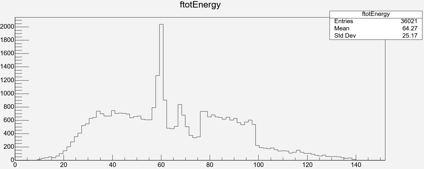
However, to get started, I wanna’ validate the simulation with the real world and the histogram created looks quite nice:
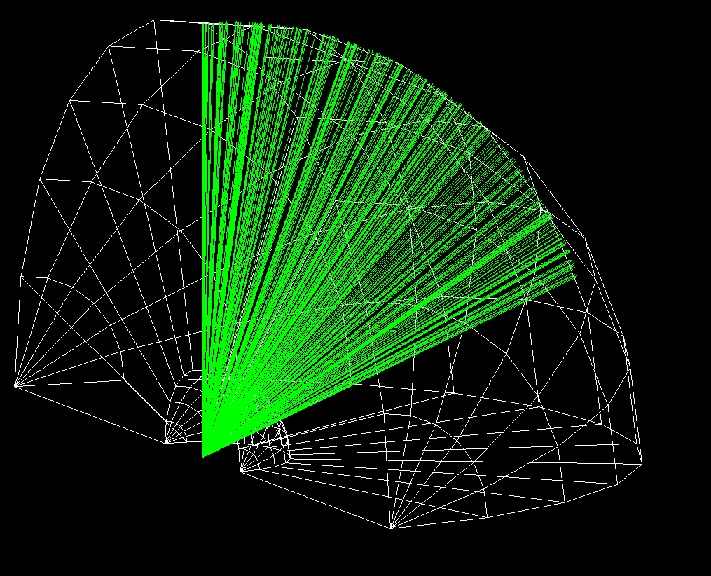
One could even say it is identical - with one difference: As you probably already noticed there is a distinctive area in the energy region from around 80 - 100 keV. What could cause this? The simulation consists here only of the particle gun and a detector:
I will happily provide more information/code, please let me know what you need.
In any case, thanks a lot already in advance!
Could there anything result from the apparent fact that the photons are apparently not killed before they reach the end of the detector?
I figured out the following, now. Firstly, the above spectrum was created with these values:
  fNPoints = 60;
  G4double xx[] =
    {
		0.01*MeV,
		0.012*MeV,
		0.014*MeV,
		0.016*MeV,
(...)
as the histogram is plotted in MeV then, I multiplied the entire array with 1000 to get keV values:
// Convert MeV to keV
for (int i = 0; i < 60; i++)
{
	xx[i] = xx[i] * 1000;
}
which wasn’t smart, I admit. So I guess the above spectrum was simulated with false energies.
Now, I’m using:
  fNPoints = 60;
  G4double xx[] =
    {
		10*keV,
		12*keV,
		14*keV,
(...)
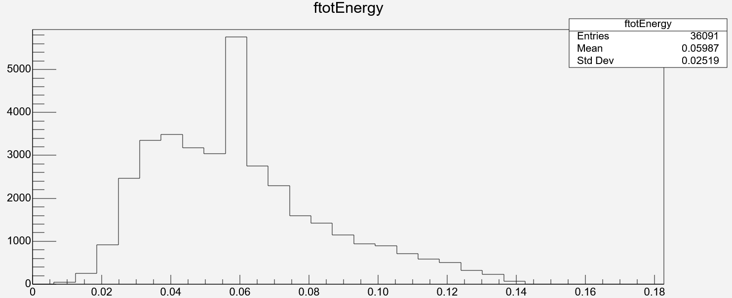
which produces the following spectrum:
which removes this suspicious region within 0.08 - 0.1 MeV. However, now it looks like the second peak vanished (I hope this is due to statistics, I’ll check this). Nevertheless, is it possible to plot the histogram in keV? It also seems that the binning changed though the entries are the same.
I figured out this now as well and the second peak vanished because of the binning, indeed.
Nevertheless, I would come back to the first question: The region from 80 - 100 MeV (very first plot above, the numbers are MeV and not keV!) shows a quite distinctive plateau. This raises two questions:
- What physics is happening there? In this region pair production is very dominant so I guess this process must be major player. Why particularly this energy region, though?
- This brings up the next question: Why and where does pair production occur? Why is there physics involved at all resp. why can we see physics processes playing a role when the simulation is only made of producing photons and detecting them after some centimeters of air?
Any idea?
The detector is built up as follows:
G4Material worldMat = nist->FindOrBuildMaterial(“G4_AIR”);
G4Sphere solidDetector_valxry = new G4Sphere(“solidDetector_valxry”, 30mm, 150mm, 0, 90deg, 0, 180deg);
logicDetector2 = new G4LogicalVolume(solidDetector_valxry, worldMat, “logicDetector2”);
G4VPhysicalVolume physDetector6 = new G4PVPlacement(0, G4ThreeVector(-53.66cm, -36cm - 1.8mm - 41.4cm, 0m), logicDetector2, “physDetector”, logicWorld, false, 6, true);