Hi everyone,
I’m posting to ask for some clarification on how to properly use the /gps/hist/point command for a particular application. My questions are listed at the end of this post. My post builds off of some related posts that have been very helpful in the past (What are these two things in below commands?, Example of Simulating GCR spectrum in Geant4, Can someone explain how to use a histogram energy spectrum as a source input for GPS).
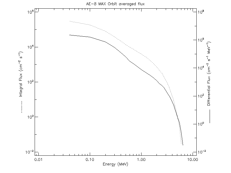
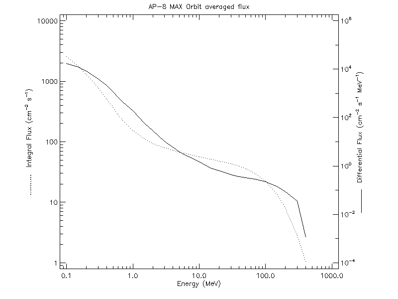
I’m attempting to irradiate a slab of material in Geant4 using protons and electrons that have energy distributions that resemble trapped protons and trapped electrons in the Earth’s radiation belts. I’ve retrieved text files from SPENVIS that contain the integral particle flux of electrons and protons at various particle energies. In Geant4, I specify the particle energy and the integral particle flux as the energy (MeV) and weight respectively in the /gps/hist/point Energy Weight command. If I plot the text files using SPENVIS, I obtain the two plots below:
Trapped Electron Data
Trapped Proton Data
I’ve read through the Geant4 documentation regarding the use of the /gps/hist/point command, however, I’m still somewhat confused on how it works. I’ve outlined my approach thus far below:
Setup Electron Source
/gps/ang/type planar
/gps/pos/type Plane
/gps/pos/shape Circle
/gps/pos/centre 0 0 20 cm
/gps/pos/radius 1 cm
/gps/particle e-
/gps/ene/type User
/gps/hist/type energy
/gps/hist/point 0 0
/gps/hist/point 0.04 302130
/gps/hist/point 0.1 185300
/gps/hist/point 0.2 80335
/gps/hist/point 0.3 39246
…
/gps/hist/point 6 0.03089
/gps/hist/point 6.5 0
/gps/hist/point 7 0
Setup Proton Source
/gps/source/add 1
/gps/ang/type planar
/gps/pos/type Plane
/gps/pos/shape Circle
/gps/pos/centre 0 0 20 cm
/gps/pos/radius 1 cm
/gps/particle proton
/gps/ene/type User
/gps/hist/type energy
/gps/hist/point 0 0
/gps/hist/point 0.1 2541.3
/gps/hist/point 0.15 1796.6
/gps/hist/point 0.2 1297.2
/gps/hist/point 0.3 786.4
…
/gps/hist/point 200 8.0887
/gps/hist/point 300 2.8558
/gps/hist/point 400 1.0349
/run/beamOn 100000
-
Since the original SPENVIS data files give the energy (MeV) vs integral particle flux data as discrete data points, I’m somewhat confused about how Geant4 uses my user-defined energy histogram. For example, in my electron source above, does Geant4 simulate the energies in between /gps/hist/point 0.04 302130 and /gps/hist/point 0.1 185300 (i.e., does Geant4 simulate the electron energies between 0.04 MeV and 0.1 MeV)? If so, is the same weight factor (i.e., 185300) applied to all energies between 0.04 MeV and 0.1 MeV?
-
From my understanding, the first /gps/hist/point command sets the lower bin edge of the histogram and the weight is automatically set to zero/is ignored by Geant4. The text files that I retrieve from SPENVIS are given as data points (i.e., not as a histogram) with the first data point being a non-zero value. And so, if I set the first /gps/hist/point command of my electron source to /gps/hist/point 0 0 and the second command to /gps/hist/point 0.04 302130, will Geant4 simulate energies between 0 MeV and 0.04 MeV with a weight of 302130?
-
This might be application-specific, but the text files from SPENVIS give both integral and differential particle fluxes. To my knowledge, Geant4 simply uses the second input into the /gps/hist/point command as the weight of the corresponding histogram bin. However, does choosing to use the integral particle flux instead of the differential particle flux as the weight in the /gps/hist/point command drastically affect the results of a Geant4 simulation? That is, is it better to use the differential particle flux instead of the integral particle flux (or vice verse) as the weight?