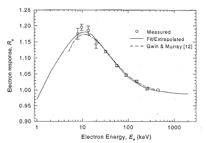
I am working on a verification test to convince myself that I am producing the correct number of scintillation photons for CsI(Tl) using the scintillation by type option to capture non-proportional scintillation yield. I want to incorporate the energy dependent electron yield data produced from Compton coincidence such as the data presented in Light yield nonproportionality of CsI(Tl), CsI(Na), and YAP | IEEE Journals & Magazine | IEEE Xplore.
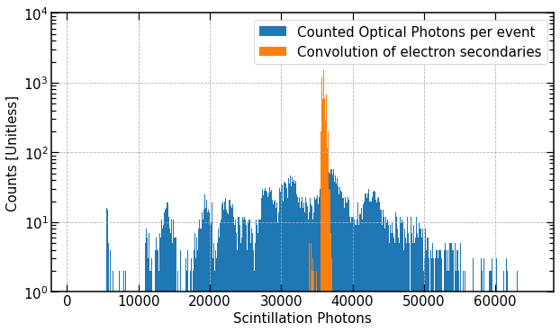
I digitized the curve above and input the x and y data as vectors for the property “ELECTRONSCINTILLATIONYIELD”. I then counted all optical photons produced per event and created a histogram from the results. I compared the optical photon per event histogram to the convolution described by equation 1 in the linked paper. If the two match then that means that the number of optical photons produced is correct.
There is a bit of difference between the two, however I believe the differences can be attributed to the fact that the author assumed no x-ray escape, difference in crystal geometry, and slightly different scaling. So I am fairly confident that my physics list sans non-proportionality and my technique for extracting and processing data is correct.
My issue is that the number of optical photons produced when I implement scintillation by type does not match the convolution, see
So my question would be, does this look like an implementation error, or is it not appropriate to use scintillation by type with the electron response plot?
I took a look at the code and it looks like the electron response plot is sampled for every step of a secondary electron, which I hope is not the case because the electron response plot should only be sample at the birth of the secondary electron. Which has me worried that I can’t use scintillation by type for non-proportional scintillation yield.
As far as I understand it, for scintillation by particle type, the values ELECTRONSCINTILLATIONYIELD are the integral of your first plot. The number of scintillation photons produced as the e- energy in a step changes from E1 to E2, is
ELECTRONSCINTILLATIONYIELD(E1) - ELECTRONSCINTILLATIONYIELD(E2).
I did a quick hand calculation to see if the integral method would work and it does not seem to be the case. I also think I may not have described how the authors intend the measured electron response to be used, so I will give that another go.
The electron response curve provides the average yield for the case that an electron fully deposited it’s energy, it is not intended to be sampled more than once for an individual electron.
Because Geant4 samples the yield at every step of the electrons path, I think that I can’t use scintillation by particle type with the typical measured electron response curves for inorganic scintillators, and that I will need to implement a custom method.
Right now my plan is to try to add an additional attribute to the particle description class that records the energy a secondary particle is born with, and to change the scintillation method to look at that birth energy when sampling from the response curve.
Well, for every process I know of in Geant4, the stepping manager gets the relevant physical properties for the current energy of the particle.
I don’t understand. Maybe you or someone else can enlighten me, for the sake of maintaining the code if nothing else. How do you go from your first figure to your third? In figure 1, say a 100 keV electron is incident–how many photons are produced? Why can’t you go from that to an ELECTRONSCINTILLATIONYIELD?
For each event I record all gamma ray interactions as well as the energy that the secondary electrons are born with. I output this data to a text file, and with Python code remove all data for events where the primary particle did not terminate with a photoelectric event, my primaries being 662 keV gammas.
For each kept event I have a list of secondary electrons energies, which I then convolute with Fig 1. To finish I sum these convoluted energies to obtain the yield for that event. That’s how I was able to generate Figure 2.
If you assume full energy deposition then you would sample Fig 1. at 100 keV and that would be your normalized yield value. The normalized yield would then have to be multiplied by a yield value you could get from a manufacturer, I used 54 gammas per keV for CsI which was information from Saint Gobain which they measured at 662 keV.
The response curves I used were normalized to one at 442 keV. When I input the response curve to Geant4 I normalized to one at 662 keV since that is the energy Saint Gobain measured their yield value.
To wrap up, we would expect on average (100)(1.04)(54)=5616 optical photons for a 100 keV electron fully depositing it’s energy in CsI. The 1.04 is the value you get from sampling Fig 1. scaled to unity at 662 keV.
Let’s say that the 100 keV electron took two steps to deposit it’s energy 10, then 90 keV, if I understand the code right Geant4 would sample Fig. 1. 100 then 90 keV, instead of just at 100 keV.
Update, one of my colleagues showed me how I was being stupid. I believe it should work out now. I think that I need to multiply the y-axis of Figure 1 with it’s x-axis then multiply by the yield at the normalized value. I will post a plot later to show how this turns out.
My confusion was that I could not stop thinking of the ELECTRONSCINTILLATIONYIELD like the scintillation yield, instead of how you described it
So I should have read your reply more closely instead of being pig-headed. That statement there is the solution to my original question, thanks for bearing with me!
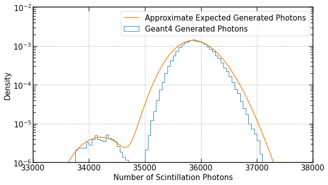
The output looked pretty good now that I have implemented ELECTRONSCINTILLATIONYIELD correctly, the shape is what I expect. I did not use Figure 2 directly for the comparison, since Figure 2 shows a histogram of mean values, with no assumption made on the variance of the distribution about said mean. I was a bit misleading in comparing the two in Figure 4 but I knew even when expanding out the expected distribution that the two would not match.
Since I defined my resolution scale to be 1 in Geant4, i.e. Poisson, I converted each bin into a Poisson distribution.
I only ran 3E5 events for this one but for the most part I think I am happy with how it turned out, I have one more check to do but I think I am done posting any updates. Again thanks to dsawkey for helping with my problem!